04. Building a Kinematic Model

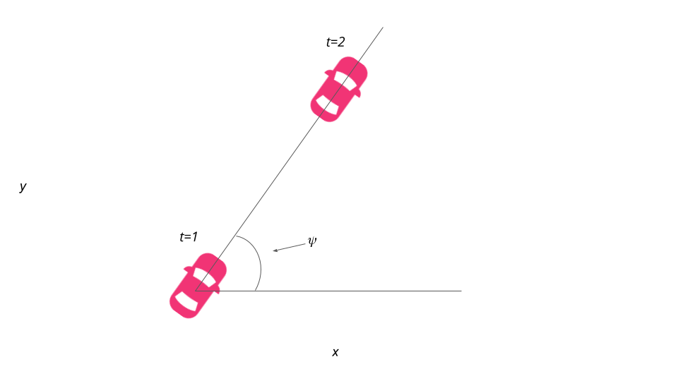
Based on the above visual answer the following quizzes:

Next, let's turn our attention to \psi :

In a nutshell, we add a multiplicative factor of the steering angle, \delta to \psi .

L_f measures the distance between the center of mass of the vehicle and it's front axle. The larger the vehicle, the slower the turn rate.

If you've driven a vehicle you're well aware at higher speeds you turn quicker than at lower speeds. This is why v is the included in the update.

Finally, let's take a look at how the velocity, v is modeled:

v = v + a*dt

where a can take value between and including -1 and 1.

Awesome! We've now defined the state, actuators and how the state changes over time based on the previous state and current actuator inputs.

Here it is:

x_{t+1} = x_t + v_t cos(\psi_t) * dt

y_{t+1} = y_t + v_t sin(\psi_t) * dt

\psi_{t+1} = \psi_t + \frac {v_t} { L_f} \delta_t * dt

v_{t+1} = v_t + a_t * dt

How L_f was chosen for this project:

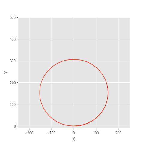
On the topic of running a vehicle around in a circle, this is actually a good way to test the validity of a model! If the radius of the circle generated from driving the test vehicle around in a circle with a constant velocity and steering angle is similar to that of your model in the simulation, then you're on the right track. This type of approach was used to tune L_f .

From the image below, we can see that the vehicle started at the origin, oriented at 0 degrees. We then simulated driving with a \delta value of 1 degree and adjusted L_f to arrive at a final value of 2.67 . This is the value that produced a circle, with all other variables held constant.